Introduction

At this point of the game, I feel like neural networks have been sort of black boxed, and for good reason. They are complex systems. Just forward and backward propagation may be hard to get your head around, but then you get into different architectures like LSTMs, self-attention, U-Nets, etc. Not to mention the heavily optimized optimizers for these neural networks to make training one as fast as possible. Even though I know the basics of the math behind these things, I still wanted to take a look inside a neural network and look at what it is actually learning so I could get an overall better understanding at what was going on.

The Model

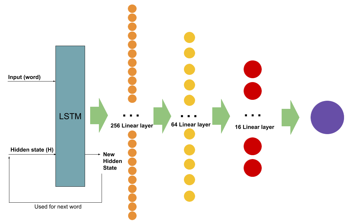
Before I can actually look inside a model, I need to make one. Although there are many different types of architecture that I could potentially do, I needed something that would be easy for me to analyze as well as have a simple architecture. I chose an LSTM (for natural language processing). There are a couple reasons, but the main one is how easy it is to analyze.  All I have to do is look at the LSTM’s state after each word. LSTMs work by incorporating a “hidden state” into the network. Think of this hidden state as a notepad for keeping track of what the LSTM has already seen. This is advantageous because instead of having to input the entire sentence into the network, we can go word by word and see how the hidden state affects the neural network for each word

Specifically, we will have an LSTM, a 256 linear layer, a 64 linear layer, a 16 linear layer, and then a sigmoid to create the final value.

I also trained the model on a basic sentiment analysis dataset based on movie reviews.

Analyzing the last layer

In order to see what's going on inside the network, let's graph the activations of the last 16 neurons (the last layer) for each word in a given sentence. Just to see what happens, we will input two sentences: “I love this movie,” and “I hate this movie.”

* Note the scale in each of the graphs. The second graph has a smaller magnitude

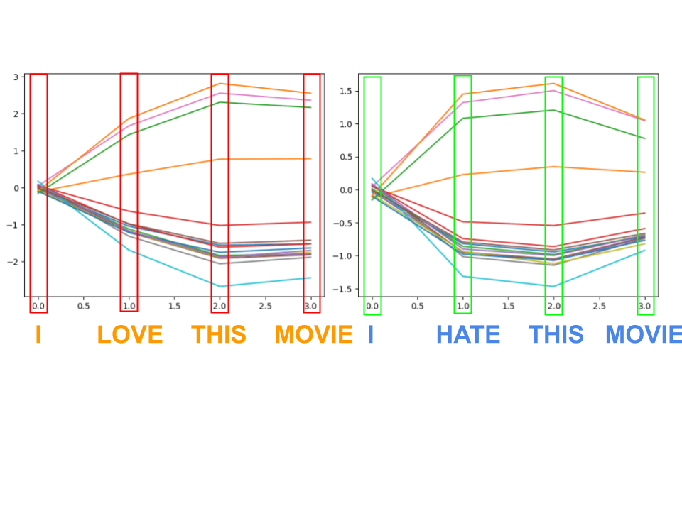
This is the graph outputted when putting these sentences through the LSTM. Remember, LSTMs work by going through the sentence one word at a time (or sometimes by word parts) and updating its hidden state based on what it has seen. This means that for each word, the activations of the last layer are going to change.

I found it quite interesting to see how the LSTM behaved when faced with different words. Even though there isn’t a large selection, you can still see some “reactions” as it reads the sentence. For example, the key words “love” and “hate” caused a huge spike. Even more interestingly, the word “this” actually caused a bigger change than “love”. Perhaps this is because “love” doesn’t necessarily mean positive sentiment, since the sentence could always switch up and say “I love how bad the CG is,” whereas the word “this” actually solidifies that the reviewer actually does love the movie, and not something bad about it.

The other very interesting thing you can find from analysis is how a lot of neurons seem to follow the exact same path -- this is indicative that the neural network actually has too many neurons to work with since many of them learn the same features. This is not ideal, but isn’t necessarily a bad thing. However, this led me to want to try and see if I can possibly reduce the amount of neurons being used. This is easily done by just retraining the network with, say, a 4 neuron linear layer rather than a 16 neuron linear layer. However, this may not be feasible for larger networks. So, the question was, how could you take this existing too-large network, and somehow compress it down into a smaller network without having to retrain the entire thing.

Compressing the Neural Network

From the last two graphs we see that there are redundancies in the features that each of the neurons in the layers are learning.

Let’s say we want to reduce the number of neurons in the last layer from 16 → 4. The simplest way to do this is to just freeze the weights of the LSTM and the other two layers and just train the 4 neurons. With just 1 epoch of training, it was able to achieve around the same accuracy of the normal model. But can we do better?

Instead of having to start from scratch, we technically have data on what the weights of the neurons should be, or in other words what the major features the neurons are going to learn. They are just duplicated and slightly changed. So, if we can somehow intelligently choose the starting weights for each of the new 4 neurons based on the redundant old 16 neurons, maybe we can reduce the amount of training needed.

Clustering the Neurons

In order to intelligently choose the starting weights, I thought it would be best to cluster them into 4 groups. Each group will contain neurons with the most similar feature. The plan is to choose one neuron from each group and then use that as the starting point for the new network to be trained.

Before we can do any kind of clustering, we need to come up with a way to compare one neuron to another. I came up with a handy algorithm to test how similar two graphs were.

1. Normalize the graph from each neuron
2. For each adjacent point, calculate the slope in each graph
3. Compare the slopes for each equivalent pair of points
4. Record a similarity value for the pair neurons
5. Repeat for every combo of neurons

This may sound confusing, but it is actually quite simple. Let’s take an example.

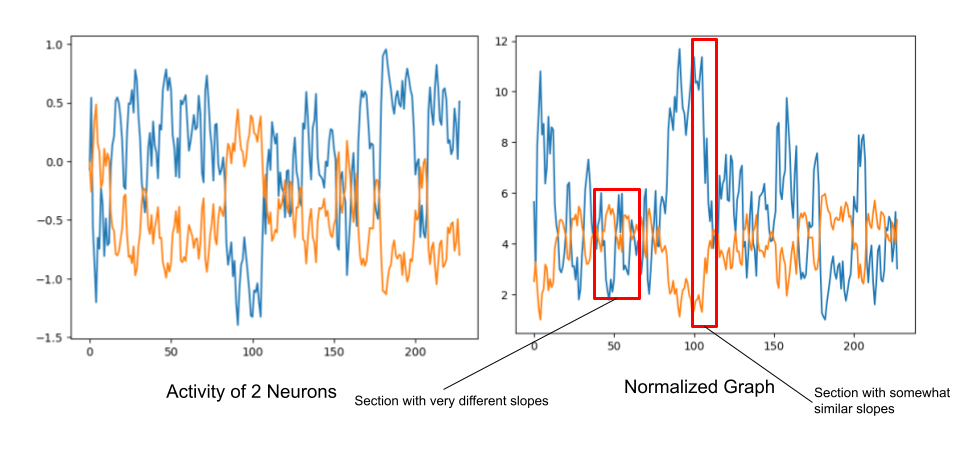
Here is the graph of two neurons. From this you can see that these two neurons create similar shapes but at a different magnitude (blue is a lot more dramatic than orange.)

Then, for each pair of neurons we would figure out the average difference among the dataset. This results in a 16x16 matrix in which each value indexed at [i, j] = similarity(i, j). This will be useful for the next step.

Now that we have a way of comparing two neurons we can cluster them. For this we will use something called Spectral Clustering. This technique is useful because it allows us to use the similarity matrix we just created between each neuron to generate the cluster. Think of clustering as a way to categorize each neuron into multiple groups, where each group contains the most similar neurons.

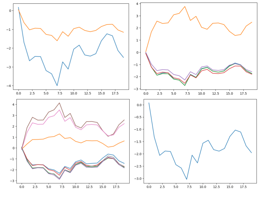
These are the neuron activations for an example sentence categorized into their respective clusters. Due to the auto-scaling of matplotlib’s plots, the scale is different on each of the graphs. For example, the top left cluster and bottom right cluster look very similar. However, the bottom right graph’s scale is different from the top left.

There are 4 clusters for each of the 4 neurons we want to turn the 16 neuron layer into. Since I specifically chose 4 clusters, you can see clusters that look like they should be together but had to be split since the algorithm was forced into making 4 clusters.

Training a better network

Now that we have clusters, we can pick one neuron from each of the clusters at random and use its weights as the starting point. The problem? It doesn’t quite work.

The problem is that for a model this simple, the network without the starting point performed as good as the one using the clusters simply because 1 epoch is more than enough to train that one layer, and there was really no accuracy gain from using the neurons as a starting point.

This was upsetting, but I had one more idea. What if we could do this neural network compression with no further training at all? It was possible if you relied on the fact that some neurons can be very close together in terms of activations.

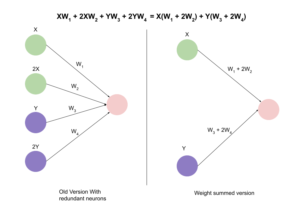
On the left, we have a neural network that has been found to have 2 clusters of similar neurons. For the green neurons, X indicates their activation. We find that one green neuron is generally double the other green neuron, in this hypothetical example. The same goes for the purple ones. Then, at the top you can see the equation that these neurons create. Simply multiply the activation by the weight. Since there is only one output, we only need one weight. However, since we know that one of the neurons is double the other, we find that we can actually factor out that common X or Y. This results in one less neuron being needed because we can just use one of them and add the weights in order to get the same result with less neurons in the layer.

In practice, the factors by which neurons differ will not be as perfect as 2. In fact, most of the time it will be closer to 1, and even then the transformation won’t technically be as accurate as using all the neurons. However, it is a close enough approximation that it should just work.

From a 79.692% accuracy baseline network, the “compressed” version using weight summing actually performed better than the re-trained version. In fact, it got a whopping 79% accuracy, which compared to the baseline is only a slight decrease.

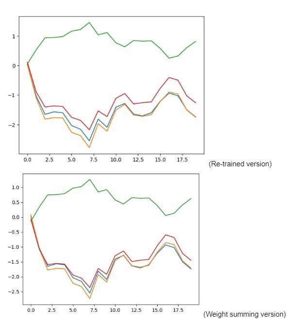
Another interesting phenomenon is that the re-trained version with the starting weights actually learned extremely similar features to the weight-summed version without training. The graphs of each can be seen below. It's fascinating to see how training the network actually came to the same conclusion as us.

Conclusion

Honestly, while this is extremely interesting, weight-summing may not even be that useful. I'm not saying that it couldn’t be, but much further testing is needed on larger models. One glaring issue is the performance of similarity matrix generation. I used a pretty badly optimized algorithm for generating it (it was quick enough that I didn’t feel the need to complicate it), but even an optimized version wouldn’t be able to handle the billions of parameters that are in models today. At that point it may be easier to just retrain the entire model with less parameters. Still, regardless of whether it could be useful, research like this is what is driving the world of artificial intelligence forward. After all, for every 1 success, 100s of people have failed in the meantime. But, that doesn’t really mean that the failures were unimportant. They are simply paving the way to success.